bench - Single Cell Modeling Tool
The single cell experimentation tool bench is quite versatile and can be used to replicate a wider range of single cell experimental protocols. A tutorial on how to use bench is given here. The following sections demonstrate how one explores all available bench functions and explains the command line arguments available.
Getting Help
The --help, --detailed-help or --full-help arguments provide a list of all available arguments with increasing levels of detail.
    bench --help

    LIMPET 1.1

    Use the IMP library for single cell experiments. All times in ms; all voltages
    in mV;  currents in uA/cm^2

    Usage: LIMPET [-h|--help] [--detailed-help] [--full-help] [-V|--version]
             [-cFLOAT|--stim-curr=FLOAT] [--stim-volt=FLOAT] [--stim-file=STRING]
             [-aDOUBLE|--duration=DOUBLE] [-DDOUBLE|--dt=DOUBLE] [-nINT|--num=INT]
             [--ext-vm-update] [--rseed=INT] [-TDOUBLE|--stim-dur=DOUBLE]
             [-A|--stim-assign] [--stim-species=STRING] [--stim-ratios=STRING]
             [--resistance=DOUBLE] [-ISTRING|--imp=STRING]
             [-pSTRING|--imp-par=STRING] [-PSTRING|--plug-in=STRING]
             [-mSTRING|--plug-par=STRING] [--load-module=STRING]
             [-lDOUBLE|--clamp=DOUBLE] [-LDOUBLE|--clamp-dur=DOUBLE]
             [--clamp-start=DOUBLE] [--clamp-SVs=STRING] [--SV-clamp-files=STRING]
             [--SV-I-trigger] [--AP-clamp-file=STRING] [-NDOUBLE|--strain=DOUBLE]
             [-tDOUBLE|--strain-time=DOUBLE] [-yFLOAT|--strain-dur=FLOAT]
             [--strain-rate=DOUBLE] [-oDOUBLE|--dt-out=DOUBLE]
             [-OSTRING|--fout=STRING] [--no-trace] [--trace-no=INT] [-B|--bin]
             [-uSTRING|--imp-sv-dump=STRING] [-gSTRING|--plug-sv-dump=STRING]
             [-d|--dump-lut] [--APstatistics] [-v|--validate]
             [-sDOUBLE|--save-time=DOUBLE] [-fSTRING|--save-file=STRING]
             [-rSTRING|--restore=STRING] [-FSTRING|--save-ini-file=STRING]
             [-SDOUBLE|--save-ini-time=DOUBLE] [-RSTRING|--read-ini-file=STRING]
             [--SV-init=STRING]
      or : LIMPET [--list-imps] [--plugin-outputs] [--imp-info]
      or : LIMPET [--stim-times=STRING]
      or : LIMPET [--numstim=INT] [-iDOUBLE|--stim-start=DOUBLE]
             [-bDOUBLE|--bcl=DOUBLE]
      or : LIMPET --restitute=STRING [--res-file=STRING] [--res-trace]
      or : LIMPET --clamp-ini=DOUBLE --clamp-file=STRING

      -h, --help                   Print help and exit
          --detailed-help          Print help, including all details and hidden
                                     options, and exit
          --full-help              Print help, including hidden options, and exit
      -V, --version                Print version and exit

     Mode: regstim
      regular periodic stimuli
          --numstim=INT            number of stimuli  (default=`1')
      -i, --stim-start=DOUBLE      start stimulation  (default=`1.')
      -b, --bcl=DOUBLE             basic cycle length  (default=`1000.0')

     Mode: neqstim
      irregularly timed stimuli
          --stim-times=STRING      comma separated list of stim times  (default=`')

     Mode: restitute
      restitution curves
          --restitute=STRING       restitution experiment  (possible
                                     values="S1S2", "dyn", "S1S2f")
          --res-file=STRING        definition file for restitution parameters
                                     (default=`')
          --res-trace              output ionic model trace  (default=off)

     Mode: info
      output IMP information
          --list-imps              list all available IMPs  (default=off)
          --plugin-outputs         list the outputs of available plugins
                                     (default=off)
          --imp-info               print tunable parameters and state variables for
                                     particular IMPs  (default=off)

     Mode: vclamp
      Constant Voltage clamp
          --clamp-ini=DOUBLE       outside of clamp pulse, clamp Vm to this value
                                     (default=`-80.0')
          --clamp-file=STRING      clamp voltage to a signal read from a file
                                     (default=`')

     Group: stimtype
      stimulus type
      -c, --stim-curr=FLOAT        stimulation current  (default=`60.0')
          --stim-volt=FLOAT        stimulation voltage
          --stim-file=STRING       use signal from a file for current stim

    Simulation control:
      -a, --duration=DOUBLE        duration of simulation  (default=`1000.')
      -D, --dt=DOUBLE              time step  (default=`.01')
      -n, --num=INT                number of cells  (default=`1')
          --ext-vm-update          update Vm externally  (default=off)
          --rseed=INT              random number seed  (default=`1')

    Stimuli:
      -T, --stim-dur=DOUBLE        duration of stimulus pulse  (default=`1.')
      -A, --stim-assign            stimulus current assignment  (default=off)
          --stim-species=STRING    concentrations that should be affected by
                                     stimuli, e.g. 'K_i:Cl_i'  (default=`K_i')
          --stim-ratios=STRING     proportions of stimlus current carried by each
                                     species, e.g. '0.7:0.3'  (default=`1.0')
          --resistance=DOUBLE      coupling resistance [kOhm]  (default=`100.0')

    Ionic Models:
      -I, --imp=STRING             IMP to use  (default=`MBRDR')
      -p, --imp-par=STRING         params to modify IMP  (default=`')
      -P, --plug-in=STRING         plugins to use, separate with ':'  (default=`')
      -m, --plug-par=STRING        params to modify plug-ins, separate params with
                                     ',' and plugin params with ':'  (default=`')
          --load-module=STRING     load a module for use with bench (implies --imp)
                                     (default=`')

    Voltage clamp pulse:
      -l, --clamp=DOUBLE           clamp Vm to this value  (default=`0.0')
      -L, --clamp-dur=DOUBLE       duration of Vm clamp pulse  (default=`0.0')
          --clamp-start=DOUBLE     start time of Vm clamp pulse  (default=`10.0')

    Clamps:
          --clamp-SVs=STRING       colon separated list of state variable to clamp
                                     (default=`')
          --SV-clamp-files=STRING  : separated list of files from which to read
                                     state variables  (default=`')
          --SV-I-trigger           apply SV clamps at each current stim
                                     (default=on)
          --AP-clamp-file=STRING   action potential trace applied at each stimulus
                                     (default=`')

    Strain:
      -N, --strain=DOUBLE          amount of strain to apply  (default=`0')
      -t, --strain-time=DOUBLE     time to strain  (default=`200')
      -y, --strain-dur=FLOAT       duration of strain (default=tonic) [ms]
          --strain-rate=DOUBLE     time to apply/remove strain  (default=`2')

    Output:
      -o, --dt-out=DOUBLE          temporal output granularity  (default=`1.0')
      -O, --fout[=STRING]          output to files  (default=`BENCH_REG')
          --no-trace               do not output trace  (default=off)
          --trace-no=INT           number for trace file name  (default=`0')
      -B, --bin                    write binary files  (default=off)
      -u, --imp-sv-dump=STRING     sv dump list  (default=`')
      -g, --plug-sv-dump=STRING    : separated sv dump list for plug-ins, lists
                                     separated by semicolon  (default=`')
      -d, --dump-lut               dump lookup tables  (default=off)
          --APstatistics           compute AP statistics  (default=off)
      -v, --validate               output all SVs  (default=off)

    State saving/restoring:
      -s, --save-time=DOUBLE       time at which to save state  (default=`0')
      -f, --save-file=STRING       file in which to save state  (default=`a.sv')
      -r, --restore=STRING         restore saved state file  (default=`a.sv')
      -F, --save-ini-file=STRING   text file in which to save state of a single
                                     cell  (default=`singlecell.sv')
      -S, --save-ini-time=DOUBLE   time at which to save single cell state
                                     (default=`0.0')
      -R, --read-ini-file=STRING   text file from which to read state of a single
                                     cell  (default=`singlecell.sv')
          --SV-init=STRING         colon separated list of comma separated
                                 SV=initial_values
Available models
The --list-imps argument outputs a list of all available ionic models and plugins.
    bench --list-imps

    Ionic models:
        AlievPanfilov
        ARPF
        Steward
        converted_COURTEMANCHE
        converted_DiFranNoble
        converted_LRDII_F
        converted_MBRDR
        converted_NYGREN
        converted_RNC
        converted_TT2
        converted_UCLA_RAB
        UCLA_RAB_SCR
        COURTEMANCHE
        DiFranNoble
        ECME
        FHN_RMcC
        FOX
        GPB
        GPVatria
        GPB_Land
        GW_CAN
        hAMr
        HH
        IION_SRC
        INADA_AVN
        Iribe
        JBTT2
        Kurata
        LMCG
        LR1
        LRDII
        LRDII_F
        MacCannell_Fb
        MitchellSchaeffer
        mMS
        MBRDR
        MurineMouse
        NYGREN
        ORd
        Pandit
        PASSIVE
        PUG
        Rat_neon
        RNC
        SC
        TT2
        TT
        TTRED
        UCLA_RAB
        WANG_NNR
        SHANNON
        GTT2_fast
        GTT2_fast_PURK
        JB_COURTEMANCHE
    Plug-ins:
        converted_EP
        converted_EP_RS
        converted_IA
        EP
        EP_RS
        ExcConNHS
        I_ACh
        IA
        IFun
        I_KATP
        INa_Bond_Markov
        I_NaH
        Muscon
        NPStress
        FxStress
        TanhStress
        Rice
        LandStress
        NHSstress
        Lumens
        SAC_KS
        YHuSAC
Show model state variables and exposed parameters
The --imp-info argument lists all state variables of a model and all exposed parameters which can be modified. For instance, to interrogate this for the tenTusscher 2 model run:
    bench --imp TT2 --imp-info

    TT2:
                                     big_cnt        0
                                       fmode        0
                                          Ko        5.4
                                         Cao        2
                                         Nao        140
                                          Vc        0.016404
                                         Vsr        0.001094
                                        Bufc        0.2
                                       Kbufc        0.001
                                       Bufsr        10
                                      Kbufsr        0.3
                                      Vmaxup        0.006375
                                         Kup        0.00025
                                           R        8314.47
                                           F        96485.3
                                           T        310
                                       RTONF        26.7138
                                 CAPACITANCE        0.185
                                         Gkr        0.153
                                        pKNa        0.03
                                         Gks        0.392
                                         GK1        5.405
                                         Gto        0.294
                                         GNa        14.838
                                        GbNa        0.00029
                                         KmK        1
                                        KmNa        40
                                        knak        2.724
                                        GCaL        3.98e-05
                                        GbCa        0.000592
                                       knaca        1000
                                       KmNai        87.5
                                        KmCa        1.38
                                        ksat        0.1
                                           n        0.35
                                        GpCa        0.1238
                                        KpCa        0.0005
                                         GpK        0.0146
                                   scl_tau_f        1
                                       flags        ENDO|EPI|MCELL
            State variables:
                                    Ca_i
                                    CaSR
                                    CaSS
                                      R_
                                       O
                                    Na_i
                                     K_i
                                       M
                                       H
                                       J
                                     Xr1
                                     Xr2
                                      Xs
                                       R
                                       S
                                       D
                                       F
                                      F2
                                   FCaSS
The --plugin-outputs argument provides the same information as --imp-info, but lists in addition all the outputs of plugins, that is, global quantities modified by a given plugins.
    Plug-ins:
            converted_EP     Iion
            converted_EP_RS  Iion
            converted_IA     Iion
            EP               Iion
            EP_RS            Iion
            ExcConNHS        Tension
            I_ACh            Iion
            IA               Iion
            IFun             Iion
            I_KATP           K_e Iion
            INa_Bond_Markov  Iion
            I_NaH            Na_e
            Muscon           Tension
            NPStress         Tension
            FxStress         Tension
            TanhStress       Tension
            Rice             Tension
            LandStress       Tension
            NHSstress        Tension
            Lumens           delLambda Tension
            SAC_KS           Iion
            YHuSAC           Iion
Define a stimulus
The arguments --stim-curr and --stim-volt select the magnitude of a current or voltage stimulus pulse in \(\mu A/cm^2\) and \(mV\), respectively. The duration of a stimulus is set through the stim-dur argument. Alternatively, a trace file can be provided through --stim-file to impose a stimulus of arbitrary shape.
To initiate an action potential in the TT2 model by applying a current stimulus of \(60 \mu A/cm^2\) and 2 ms duration run
bench --stim-curr 60 --stim-dur 2or, to stimulate with an arbitrary stimulus current profile run
bench --stim-file mypulse.trcwhere the stimulus definition file mypulse.trc must comply with the following format:
   #samples
   t0  y0
   t1  y1
   t2  y2
   ...
   tN  yN
Define a stimulus protocol
Two types of protocols are supported, a train of regular periodic stimuli or a train of irregularly time stimuli. In the regular case the total number of stimuli to be delivered is prescribed by --numstim and the interval between stimuli by the basic cycle length argument --bcl. The stimulus protocol is initiated at a given time prescribed by --stim-start.
bench --imp TT2 --numstim 50 --stim-start 10. --bcl 350An irregular stimulus sequence is specified through the --stim-times argument.
bench --imp TT2 --stim-times 10,360,700,920The response to this stimulus definition is illustrated here. When using the --stim-times options the number of stimuli depends solely on the times provided, using the --num-stim causes a conflict.
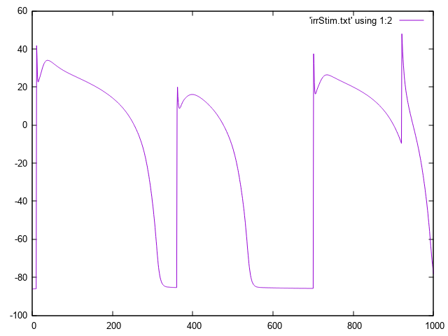
--stim-times. Read the default command line output
Depending on the ionic model and the plugins used global variables which may diffuse at the tissue level are written to the console. The output will look similar to
   bench --imp TT2

   Outputting the following quantities at each time:
      Time              Vm            Iion

     0.000 -8.62000000e+01 +0.00000000e+00
     1.000 -8.61618521e+01 -3.46181728e-02
     2.000 +4.10176938e+01 -6.35646133e+01
     3.000 +3.51969845e+01 +1.22923870e+01
     4.000 +2.62015535e+01 +5.84205961e+00
     5.000 +2.29077661e+01 +1.52032351e+00
   ...
To quickly visualize AP shape or ionic current redirect the output to a file and visualize with your preferred tool.
Basic stimulation control
The overall duration of simulation is set by --duration in [ms] and the integration time step is chosen by --dt in [ms]. The time stepping method cannot be chosen at the command line as ODE integration in LIMPET is hardcoded, but the source code for any ionic model can be regenerated with a different integration scheme (see limpet_fe.py for details). To simulate 10 action potentials at a basic cycle length of 500 ms the overall duration of the simulation should be picked as :math:10 \times 500 ms = 5000 ms.
bench --duration 5000 --bcl 500 --num-stim 10 --stim-start 0Simple AP visualization
To quickly visualize the shape of an action potential or the ionic current redirect the output to a file
bench --duration 400 --dt-out 0.1 --fout=APTime \(t\), transmembrane voltage \(V_{\mathrm m}\)and ionic current, $I_{\mathrm {ion}}$ are written to the fileAP.txt. Use your favourite plotting tool such as, for instance,gnuplot`.
   gnuplot

   # plot Vm
   plot 'AP.txt' using 1:2 with lines

   # plot Iion
   plot 'AP.txt' using 1:3 with lines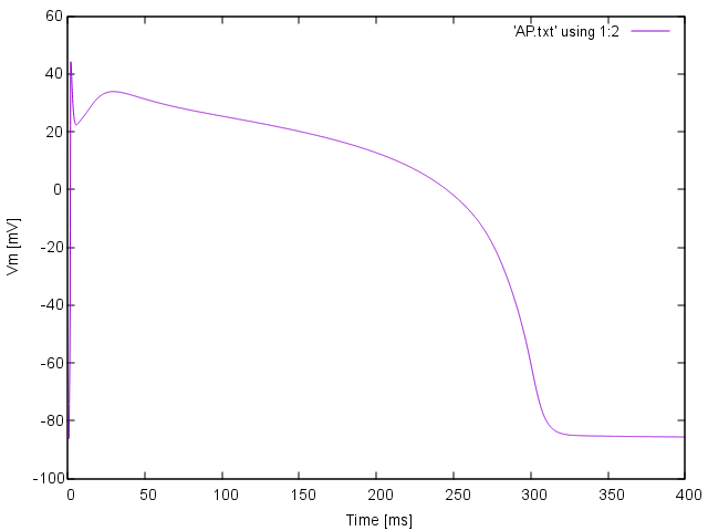
Performance benchmarking
For the sake of performance benchmarking the number of cell solved can be increased using --num. Performance metrics of the ODE solver are reported in any simulation run at the end of the output. To run a short benchmark simulating 10 ms of activity in 10000 cells use:
mpiexec -n 16 bench --num 100000 --duration 10 This outputs a basic performance statistics as shown below:
   setup time          0.001208 s
   initialization time 0.036891 s
   main loop time      2.801997 s
   total ode time      2.788086 s

   mn/avg/mx loop time 2.064943 2.799198 5.839109 ms
   mn/avg/mx ODE time  2.063036 2.785301 5.825996 ms
   real time factor    0.003587
Model modification
Model behavior can be modified by providing parameter modification string through --imp-par. Modifications strings are of the following form:
param[+|-|/|*|=][+|-]###[.[###][e|E[-|+]###][\%]where param is the name of the parameter one wants to modify such as, for instance, the peak conductivity of the sodium channel, GNa. Not all parameters of ionic models are exposed for modification, but a list of those which are can be retrieved for each model using imp-info. As an example, let's assume we are interested in specializing a generic human ventricular myocyte based on the ten Tusscher-Panfilov model to match the cellular dynamics of myocytes as they are found in the halo around an infarct, i.e. in the peri-infarct zone (PZ). In the PZ various current are downregulated. Patch-clamp studies of cells harvested from the peri-infract zone have reported a 62% reduction in peak sodium current, 69% reduction in L-type calcium current and a reduction of 70% and 80% in potassium currents \(I_{\mathrm {Kr}}\) and \(I_{\mathrm K}\), respectively. In the model these modifications are implemented by altering the peak conductivities of the respective currents as follows:
   # all modification strings yield the same results
   bench --imp TT2 --imp-par="GNa-62%,GCaL-69%,Gkr-70%,GK1-80%" --numstim 10 --bcl 500 --duration 5000

   # or
   bench --imp TT2 --imp-par="GNa*0.38,GCaL*0.31,Gkr*0.3,GK1*0.2" --numstim 10 --bcl 500 --duration 5000
To make sure that the provided parameter modifications are used as expected look at the log messages printed to the console. You should see messages confirming the use of the specified parameter modifications:
   Ionic model: TT2
           GNa                  modifier: -62%            value: 5.63844
           GCaL                 modifier: -69%            value: 1.2338e-05
           Gkr                  modifier: -70%            value: 0.0459
           GK1                  modifier: -80%            value: 1.081
To observe the effect of the modification relative to the baseline model simulate a train of action potentials with both baseline and modified model. Run
   # run baseline model
   bench --imp TT2 --numstim 10 --bcl 500 --duration 5000 --fout=TT2_baseline

   # run modified PZ model
   bench --imp TT2 --imp-par="GNa-62%,GCaL-69%,Gkr-70%,GK1-80%" --numstim 10 --bcl 500 --duration 5000 --fout=TT2_PZ
The figure below illustrates the effect of the parameter modifications upon AP features.

Model augmentation
Published models of cellular dynamics are not complete and comprehensive representations of the electrophysiological behavior of a myocyte. Rather, the represent a subset of features which were deemed relevant for a given purpose. This is true for any published model, none of them is able to represent myocyte behavior under an arbitrary range of experimental circumstances. For the sake of verification it is crucial to be able to run models under the exact same conditions under which published results were obtained. However, after verification it is often necessary to augment a model with additional features which remained unaccounted for in the original publication. The --plug-in mechanism is designed for such applications where additional currents or physical effects such as the generation of active tension are considered without recompiling or directly modifying the model as published. The underlying concept is illustrated in this figure. Typical augmentation is used for incorporating additional currents which play a role when driving the transmembrane potential \(V_{\mathrm m}\) beyond the physiological range during the application of a strong depolarizing/hyperpolarizing stimuli such as an electroporation current, EP, an electroporation current with pore resealing, EP_RS, or a hypothetical time-independent outward rectifying potassium current IA, or to account for the effect of adrenergic stimulation by incorporating an acetylcholine-dependent potassium current I_ACh.

For instance, to augment a model of cellular dynamics to be used for studying the effect of defibrillation shocks, one would activate the plugins EP_RS and IA. This is achieved as follows:
bench --imp TT2 --plug-in "EP_RS:IA"A frequent use of plugins is the augmentation with active stress models. For instance, to specialize a human ventricular myocyte model for use in a ventricular electro-mechanical modeling study one would enable an active stress model such as LandHumanStress:
bench --imp TT2 --plug-in "LandHumanStress"As shown above in the Section on usage of --imp-par, the default behavior of plugins can also be modified in the same way as for the parent cell model. For instance, to reduce the peak force generated by 25 % one would use a plug-par string as follows:
bench --imp TT2 --plug-in "LandHumanStress" --plug-par="Tref-25%"When using more than one plugin, parameter modification strings for the various plugins are separated by a :. For instance, if we further augment with the ATP-sensitive potassium current I_KATP and modify the $f_{\mathrm ATP}).
bench --imp TT2 --plug-in "I_KATP:LandHumanStress" --imp-par "GNa*0.8" --plug-par "f_ATP-10%:Tref-10%,TRPN_n+25%"Again, a message is printed to the console confirming that the requested parameter modifications have been performed:
   Ionic model: TT2
           GNa                  modifier: *0.8            value: 11.8704
   Plug-in: I_KATP
           f_ATP                modifier: -10%            value: 0.00099
   Plug-in: LandHumanStress
           Tref                 modifier: -10%            value: 108
           TRPN_n               modifier: +25%            value: 2.5
Limit cycle
Action potentials and the trajectory of state variables depend on the basic cycle length by which myocytes are activated. Typically, a train of pacing pulses of a certain length are required until the electrical activity in a myocyte arrives at a limit cycle, that is, the transmembrane voltage \(V_{\mathrm m}(t)\) and all state variables in the state vector \(\boldsymbol{\eta}(t)\) traverse the exact trajectory in the state space after each perturbation with the same stimulus. Mathematically, this boils down to
\( \begin{equation} \boldsymbol{\eta}(t+T) = \boldsymbol{\eta}(t) \hspace{1cm} \forall t > t_{\mathrm lc} \nonumber \end{equation} \)
where \(T\) is the basic cycle length, bcl, and \(t_{\mathrm lc}\) is an instant in time beyond which we deem the time evolution of the state variables to follow a limit cycle. In general, more recent ionic models, particularly those which allow intracellular ionic concentrations to vary, are unlikely to arrive at a stable limit cycle. Instead of demanding the exact same trajectories are traversed in each cycle one could use various norms to demand that the beat-to-beat deviations in the state space remain within a certain limit, \(\delta\). For instance, we could demand
\( \begin{equation} \frac{1}{T} \int_{t}^{t+T} \frac{|| \boldsymbol{\eta}(t+T) - \boldsymbol{\eta}(t) ||}{|| \boldsymbol{\eta}(t) ||} \, dt < \delta \hspace{1cm} \forall t > t_{\mathrm lc} \nonumber \end{equation} \)
which would the relative difference between two cycles is, on average, less than a desired relative error \(\delta\). Under this norm it is still possible that relative differences exceed
While using norms to detect the instant \(t_{\mathrm lc}\) beyond which the state trajectories traverse a stable limit cycle is certainly feasible, one has to keep in mind that various myocyte models will not arrive at a stable limit cycle in the strict mathematical sense and that myocytes in vivo never operate in a regime that would comply with such a rigorous constraint. A more pragmatic approach is to determine \(t_{\mathrm lc}\) by visual inspection. This is easily achieved with limpetGUI by pacing a cell for a sufficiently larger number of pacing cycles and simply observe the envelope of all state time traces. For the purpose of illustration an example is shown in figures limit cycle envelope and limit cycle zoom.
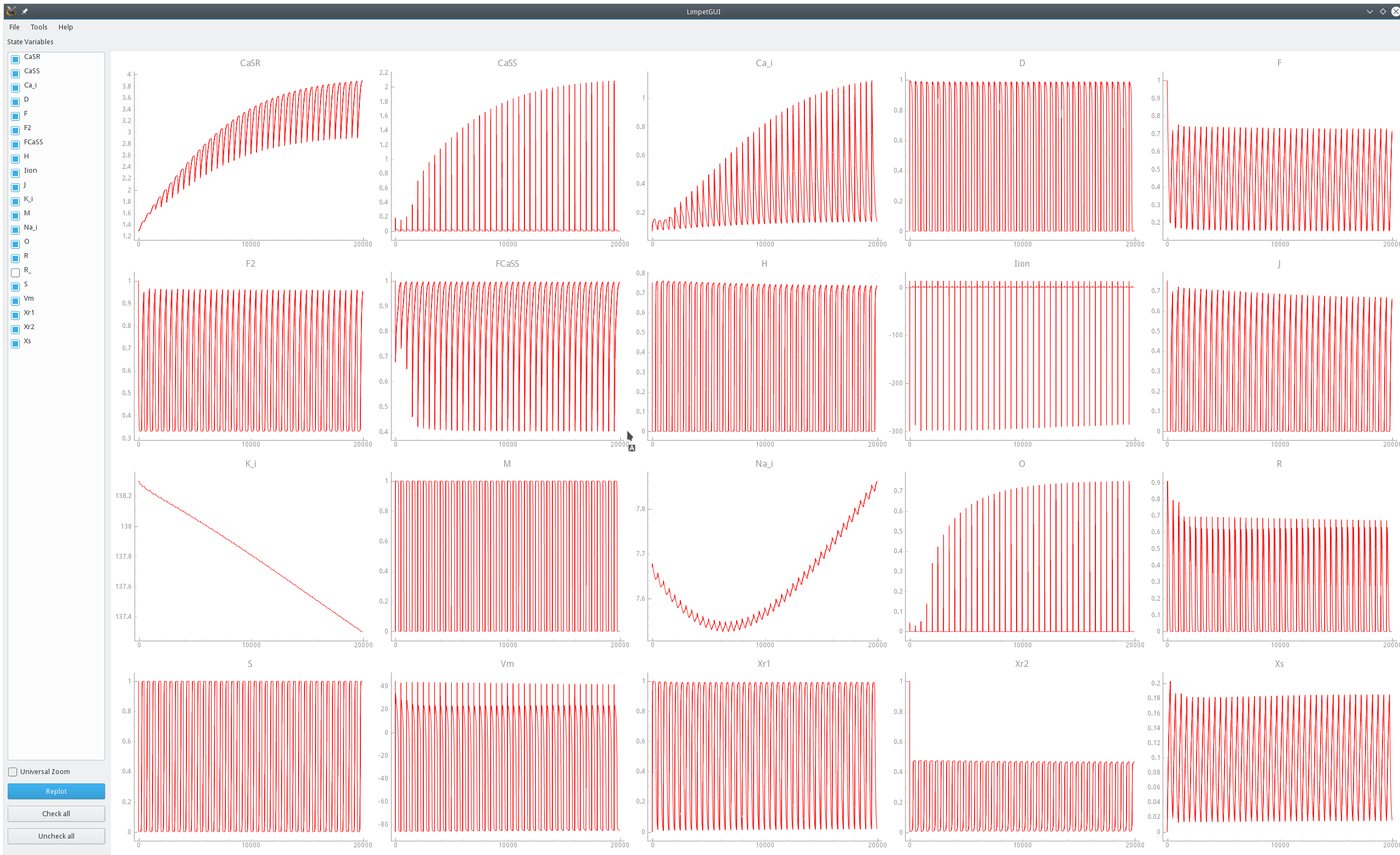
Visualization of a limit cycle pacing experiment using limpetGUI. After 20 seconds pacing at a bcl of 500 ms most state variables settle in at a limit cycle with the exception of intracellular concentration of sodium and potassium ions.
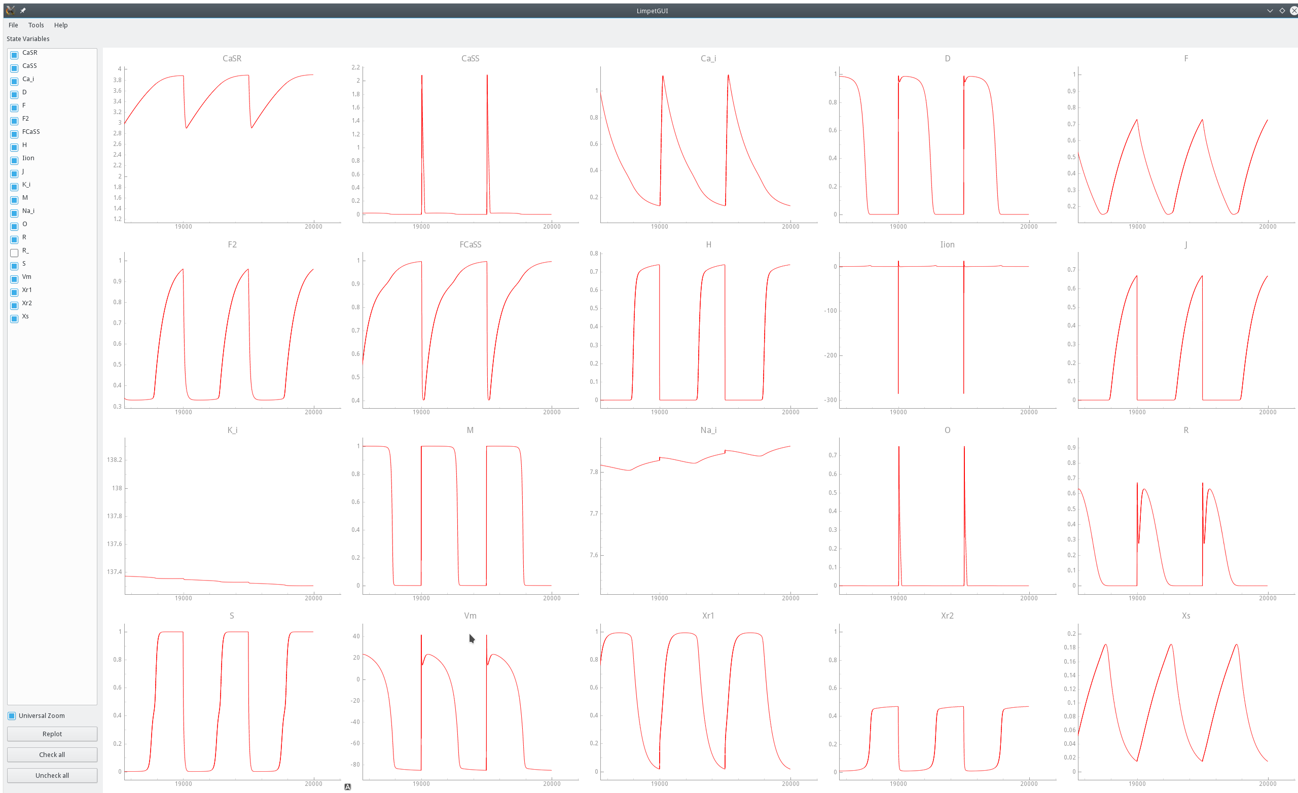
Zoom on state traces over the last three pacing cycles of the same pacing experiments shown above in figure limit cycle envelope.
Initial Cell State
Models of cellular dynamics are virtually never used with the values given for the initial state vector. Rather, cells are based to a given limit cycle to approximate the experimental conditions one is interested in. The state of the cell can be frozen at any given instant in time and this state can be reused then in subsequent simulations as initial state vector. Typically, the state of a cell is frozen in its limit cycle right at the end of the last diastolic interval. The standard procedure based on bench would proceed along the following steps:
-
Parameterize and augment a cell model corresponding to the experimental conditions of interest and for the intended application
-
Run bench then for a sufficiently large number of pacing pulses
numstimuntil a reasonable approximation of a stable limit cycle is achieved for the given cycle lengthbcl. Confirm the arrival at a limit cycle at least visually using limpetGUI. -
Store the initial state vector at the very end of the pacing protocol, that is, for
numstimstimuli and a givenbcldetermine the end time of the pacing protocol astsave = tstart + bcl*numstim -
Save the state vector at the determined time
tsaveinto a state vector file.
The last step of saving the state vector is triggered using the parameters --save-ini-time and --save-ini-file. If we want to save the state of a myocyte after 25 pacing pulses at a basic cycle length of 500 ms with the time of delivering the first pacing pulse at 0 ms one saves the initial state vector as follows:
   # run baseline model
   bench --imp TT2 --plug-in "LandHumanStress" --fout=TT2_baseline \
         --stim-start 0. --numstim 25 --bcl 500 --duration 12500 \
         --save-ini-time 12500 --save-ini-file TT2_lc_bcl_500_baseline.sv

   # run modified PZ model
   bench --imp TT2 --plug-in "LandHumanStress" --imp-par="GNa-62%,GCaL-69%,Gkr-70%,GK1-80%"  --fout=TT2_PZ \
         --stim-start 0. --numstim 25 --bcl 500 --duration 12500 \
         --save-ini-time 12500 --save-ini-file TT2_lc_bcl_500_PZ.sv
These runs generate two state vector files, TT2_lc_bcl_500_baseline.sv and TT2_lc_bcl_500_PZ.sv which store the state of each state variable at the instant t=12500 ms under the above given pacing protocol. For instance, the state vector under baseline conditions in the file TT2_lc_bcl_500_baseline.sv will be similar to:
   -85.2262            # Vm
   1                   # Lambda
   0                   # delLambda
   0.308053            # Tension
   -                   # K_e
   -                   # Na_e
   -                   # Ca_e
   0.00256503          # Iion
   -                   # tension_component
   TT2
   0.126796            # Ca_i
   3.62845             # CaSR
   0.000380231         # CaSS
   0.907029            # R_
   2.68967e-07         # O
   7.62609             # Na_i
   137.689             # K_i
   0.00172638          # M
   0.743346            # H
   0.678447            # J
   0.0150679           # Xr1
   0.470865            # Xr2
   0.0143382           # Xs
   2.43132e-08         # R
   0.999995            # S
   3.3857e-05          # D
   0.729795            # F
   0.959628            # F2
   0.995618            # FCaSS

   LandHumanStress
   0.0249847           # TRPN
   0.999196            # TmBlocked
   0.000641671         # XS
   8.33073e-05         # XW
   0                   # ZETAS
   0                   # ZETAW
   0                   # __Ca_i_local
Action Potential Duration (APD) Restitution Experiments
The single cell EP tool bench provides built-in capabilities for performing restitution experiments. Restitution experiments with bench are steered through the following command line arguments --restitute, --res-file and --res-trace.
   --restitute
                pick the protocol for performing the restitution experiment.
                Possible values are "S1S2", "dyn" or "S1S2f".

   --res-file
                definition file for restitution parameters.
                For a description of restitution file formats see :ref:`restitution protocol definition <restitution-protocol-def>`.
                By default no restitution protocol defintion file is provided.

   --res-trace
                Can be on or off, toggles writing of trace files
Action potential analysis data are written in the following format:
    #Beat Pre(P||*) lc  APD(n)  DI(n)   DI(n-1)  Tri   VmMax   VmMin

    1     *          0  288.95  711.04   11.69   0.00  44.30  -86.08
    2     *          0  286.97  713.02  711.04   0.00  45.27  -86.04
    3     *          0  288.58  711.42  713.02   0.00  45.31  -86.01
    4     *          0  304.53  695.00  711.42  78.29  45.37  -85.98
    5     *          0  305.50  694.50  695.00  78.54  45.26  -85.95
    6     *          0  305.90  694.10  694.50  78.74  45.31  -85.92
    7     *          0  306.26  693.74  694.10  78.93  45.33  -85.90
    8     *          0  306.59  693.40  693.74  79.11  45.20  -85.87
where the column headers refer to: #Beat - the total beat number in the protocol; Pre - whether beat was premature P or not ***; lc - whether AP traversed a limit cycle in the state space, 1, or not, 0; DI(n) - diastolic interval in ms of the current beat and DI(n-1) of the previous beat; Tri - Triangulation of the AP; VmMax and VmMin - maximum and minimum value of AP within pacing cycle.
Restitution data are written following the same format, but keeping only those beats which were marked as premature in the AP analysis file.
   33    P          0  276.07  723.94  180.25  85.35  41.02  -85.58
   46    P          0  272.73  727.27  170.63  85.93  40.11  -85.53
   59    P          0  268.79  731.22  161.30  86.36  39.19  -85.49
   72    P          0  264.53  735.47  151.97  86.84  38.27  -85.46
   85    P          0  259.94  740.07  142.59  87.34  37.29  -85.43
   98    P          0  255.01  744.99  133.16  87.94  36.20  -85.40
   111   P          0  249.66  750.35  123.70  88.61  35.02  -85.37
   124   P          0  243.87  756.14  114.14  89.45  33.68  -85.35
   137   P          0  237.56  762.45  104.56  90.45  32.18  -85.32
   150   P          0  230.68  769.32   94.94  91.71  30.47  -85.30
For an introduction into using :ref:bench <bench> as a tool for measuring restitution curves see the restitution experiments in the tutorials.
Code Generation
A tutorial on using the code generation tool limpet_fe.py is given here.